Introduction
Time-series data is generated whenever measurements or observations are collected over time. Examples include hourly temperatures, daily website traffic, stock prices, electricity consumption, medical measurements, and sensor readings from industrial equipment. Machine learning systems use these sequences to identify patterns, forecast future values, detect unusual behavior, and support automated decisions.
In an ideal dataset, observations arrive at consistent intervals, every expected value is available, and timestamps accurately represent when measurements occurred. Real-world data rarely meets all these conditions. Sensors may stop transmitting, users may skip measurements, financial markets may close, medical tests may be performed at irregular intervals, and data pipelines may experience delays or failures.
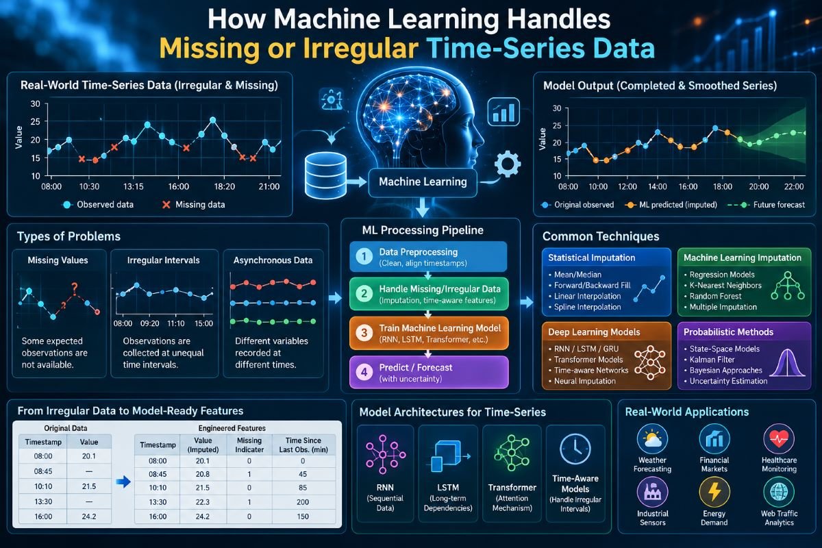
These problems create two related challenges: missing values and irregular time intervals. A missing value means an expected observation is unavailable, while irregular sampling means the time between observations varies. A dataset can contain one problem without the other, or both simultaneously.
Machine learning systems must account for these differences before they can reliably learn temporal relationships. Simply replacing missing values with averages or treating every row as equally spaced can remove important information and introduce misleading patterns.
Modern approaches combine statistical imputation, time-aware feature engineering, sequence models, probabilistic methods, and specialized architectures designed to work with incomplete observations. The appropriate method depends on the reason data is missing, the frequency of observations, the forecasting objective, and the consequences of making an incorrect prediction.
Understanding these techniques reveals how AI systems transform imperfect chronological records into useful predictions without assuming that every observation is complete or equally spaced.
Understanding Missing and Irregular Time-Series Data
Before choosing a machine learning technique, it is important to distinguish the different types of time-series problems.
Missing values
A missing value occurs when an expected measurement is not available. For example, a weather station may record temperatures at 9:00 AM, 10:00 AM, and 12:00 PM but have no reading for 11:00 AM.
The missing observation could result from a sensor malfunction, a network interruption, a failed database operation, or an intentional decision not to collect a measurement.
Missing values may appear as empty fields, null values, special markers, or absent records. These representations need to be identified during data preparation.
Irregular sampling
Irregular sampling occurs when observations are collected at unequal time intervals.
Consider these measurements:
| Timestamp | Measurement |
| 09:00 | 18.2 |
| 09:05 | 18.5 |
| 09:25 | 19.1 |
| 10:10 | 20.0 |
The intervals are five, twenty, and forty-five minutes. A model that assumes each row represents an equal time step may incorrectly interpret the changes.
Irregular sampling is not necessarily an error. A medical professional may take a measurement only when needed, or an event-based sensor may record data only when a threshold is crossed.
Delayed and asynchronous observations
A related problem occurs when measurements are collected at different times across multiple variables.
For example, a monitoring system might record temperature every minute, pressure every ten minutes, and maintenance events only when they occur. These data streams are asynchronous because their observation schedules differ.
Combining them into one dataset requires a strategy for aligning timestamps without introducing false precision.
Why the distinction matters
Missing values concern the availability of observations. Irregular sampling concerns their timing. Treating both problems as ordinary empty cells can cause a model to lose information about when the data was collected.
A reliable pipeline should preserve both the observed values and the timing information associated with them.
Why Time-Series Data Becomes Incomplete
The reason data is missing can influence which machine learning approach is appropriate.
Technical failures
Sensors can lose power, networks can disconnect, and data collection systems can experience outages. In these situations, missing observations may reflect technical problems rather than changes in the underlying process.
A long period without measurements might indicate a failed device rather than a stable environmental condition.
Human behavior
In applications involving people, observations may depend on whether someone chooses or is able to provide information.
For example, a person may record health measurements more frequently when symptoms worsen. The missingness pattern can therefore be related to the condition being monitored.
Event-driven measurement
Some systems collect measurements only when something happens. Financial transactions, machine alarms, website interactions, and emergency visits are examples of event-based data.
Periods without records may indicate that no event occurred, but this interpretation is valid only when the collection system reliably records every relevant event.
Operational schedules
Many time series naturally contain gaps. Electricity usage may follow business operating hours, markets may close on weekends, and industrial equipment may be inactive during maintenance periods.
A model must distinguish these expected gaps from unexpected data loss.
Missingness mechanisms
Statistical analysis commonly distinguishes three missing-data mechanisms.
Missing completely at random (MCAR): The probability that a value is missing does not depend on observed or unobserved data.
Missing at random (MAR): The probability of missingness may depend on information that is observed, such as a device type or previously recorded measurement.
Missing not at random (MNAR): Missingness depends on the unavailable value itself or on other unobserved information.
These categories are useful for understanding assumptions, although real datasets may not fit neatly into one category. The mechanism is often difficult to establish from the observed data alone.
For example, if a sensor fails more frequently at extreme temperatures, the missingness may be informative. Treating the gaps as random could bias the model's estimates.
Data Preparation Before Machine Learning
Effective handling of incomplete time series begins before the model is trained.
Validate timestamps
The first step is to verify that timestamps can be interpreted consistently. Problems may include invalid date formats, duplicated timestamps, inconsistent time zones, and incorrect ordering.
For data collected across regions, local timestamps may need to be converted into a consistent reference such as Coordinated Universal Time (UTC), while retaining the information required to reconstruct local time.
Daylight saving transitions can also produce repeated or nonexistent local clock times. These cases should be resolved using appropriate time-zone rules.
Sort observations chronologically
Many time-series algorithms depend on the order of observations. Data should be sorted by timestamp within each individual series before calculating differences, rolling statistics, or lagged features.
Sorting is especially important when records arrive late or are merged from several sources.
Identify duplicate records
Duplicate timestamps can indicate repeated transmissions, multiple measurements taken at the same moment, or data-processing errors.
The correct treatment depends on the meaning of the measurements. Some duplicates may be averaged, while others should be preserved as separate events or resolved using source-specific identifiers.
Measure the sampling interval
A useful diagnostic is to calculate the time difference between consecutive observations:
[\Delta t_i = t_i-t_{i-1}]
Here, (t_i) is the timestamp of the current observation and (t_{i-1}) is the previous timestamp.
Examining the distribution of (\Delta t_i) helps identify the typical sampling interval, long gaps, and unexpected changes in collection frequency.
Create a data-quality profile
Before selecting a model, analysts should measure the percentage of missing values, the length of missing intervals, the number of irregular gaps, and the availability of each variable.
This profile helps determine whether simple imputation is sufficient or whether the missingness pattern requires a more specialized method.
Traditional Methods for Filling Missing Values
Not every time-series problem requires a complex neural network. Simple statistical techniques remain useful when their assumptions are appropriate.
Mean and median imputation
Mean imputation replaces missing values with the average of observed measurements. Median imputation uses the middle value after the observations are ordered.
These methods are easy to implement and can serve as baseline approaches. However, they ignore the temporal structure of the data.
If temperatures rise throughout the day, replacing a missing afternoon value with the overall average may underestimate the actual temperature. Mean imputation can also reduce the apparent variability of a series.
Forward fill
Forward fill replaces a missing observation with the most recent previously observed value.
For example:
| Time | Original value | Forward-filled value |
| 10:00 | 12 | 12 |
| 10:05 | Missing | 12 |
| 10:10 | Missing | 12 |
| 10:15 | 15 | 15 |
This method is useful when a variable is expected to remain stable until updated, such as a configuration setting or a recorded status.
It is less suitable for rapidly changing measurements. Long forward-filled intervals can make a series appear artificially constant.
Backward fill
Backward fill uses the next available observation to fill a gap.
Although this can be appropriate in retrospective data preparation under certain assumptions, it can introduce future information into a model that is intended to make real-time predictions.
For forecasting, information from after the prediction time must not be used to construct input features.
Linear interpolation
Linear interpolation estimates missing values by drawing a straight line between two observed points.
If a measurement is 10 at time (t_1) and 16 at time (t_2), an estimate at time (t) between them can be calculated as:
[\hat{x}(t)=x_1+\frac{t-t_1}{t_2-t_1}(x_2-x_1)]
This formula accounts for the actual timestamps, making it more suitable for irregular observations than interpolation based only on row positions.
However, interpolation assumes a reasonably smooth change between the observed points. It can be misleading when the underlying process changes abruptly or contains sudden events.
Spline interpolation
Spline interpolation fits smooth curves through observed points. It can capture gradual changes more flexibly than straight-line interpolation.
However, spline methods may overshoot near boundaries or around sharp changes. They should not automatically be treated as more accurate simply because they produce smoother curves.
Choosing a baseline
The simplest method that matches the data-generating process is often a useful starting point. Baseline methods are fast, interpretable, and provide a benchmark against which more complex machine learning models can be evaluated.
How Machine Learning Improves Missing-Value Estimation
Machine learning approaches can use relationships among variables, previous observations, seasonal patterns, and other contextual information to estimate missing values.
Unlike simple imputation, these methods can learn complex relationships from historical data. Their effectiveness depends on the amount of available training data and whether the historical patterns remain relevant.
Regression-based imputation
A regression model predicts a missing variable using other available features.
For example, if an industrial system records temperature, pressure, and energy consumption, a model may learn relationships among these measurements. When one temperature value is missing, the other variables can help estimate it.
The method is most useful when the input features contain meaningful information about the missing variable.
However, relationships learned from historical observations may change under new operating conditions. Imputed values should therefore be evaluated rather than assumed to be correct.
K-nearest neighbors imputation
K-nearest neighbors (KNN) imputation identifies observations with similar characteristics and uses them to estimate missing values.
Similarity may be based on other variables, recent history, seasonal features, or a combination of factors.
For time-series data, the definition of similarity is especially important. Two observations that have similar values but occur in different seasons or operating conditions may not be suitable substitutes.
KNN can be computationally expensive for large datasets and may struggle when the available features are themselves highly incomplete.
Random forest imputation
Random forests combine multiple decision trees to learn nonlinear relationships between variables. They can estimate missing values by using patterns found in complete or partially complete records.
Such models can capture interactions that a simple linear method may miss. They are particularly useful when a dataset contains many related variables.
However, random forests do not automatically understand the order of time. Temporal features, lagged measurements, and appropriate training procedures may be needed to preserve chronological relationships.
Multiple imputation
Multiple imputation creates several plausible versions of an incomplete dataset rather than treating a single estimate as unquestionably correct.
Each completed dataset is analyzed, and the results are combined according to the relevant statistical procedure.
This approach helps represent uncertainty about missing values, particularly in statistical analyses where that uncertainty affects the conclusions.
It is more involved than single-value imputation and requires careful implementation. For forecasting systems, the appropriate method depends on whether uncertainty estimates or a single operational prediction are required.
Deep Learning for Incomplete Time Series
Deep learning can model complex temporal relationships, especially when large amounts of historical data are available.
However, a neural network does not automatically solve missing-data problems. Its architecture and input representation must be designed to handle incomplete observations correctly.
Recurrent neural networks
Recurrent neural networks (RNNs) process sequences while maintaining a representation of previous observations. Long short-term memory (LSTM) networks and gated recurrent units (GRUs) are commonly used variants designed to capture temporal dependencies.
For incomplete time series, these networks can use imputed values along with missingness indicators and elapsed-time features.
A standard RNN may perform poorly when gaps are long or sampling intervals vary significantly unless these conditions are explicitly represented.
Time-aware recurrent models
Time-aware models incorporate information about the interval since the previous observation. Rather than treating every sequence step as equally spaced, they can adjust their representations according to the elapsed time.
For example, two temperature readings separated by one minute provide different temporal context from two readings separated by six hours.
Time-aware designs can be useful for healthcare monitoring, sensor systems, and other applications with uneven sampling schedules.
Transformer-based models
Transformers use attention mechanisms to learn relationships among different positions in a sequence.
For time-series applications, timestamps, positional information, and missingness indicators can help the model understand temporal context. Some architectures are designed specifically to work with irregular observations.
However, attention alone does not guarantee correct handling of missing values. If the input representation ignores elapsed time or confuses padding with genuine measurements, the model may learn misleading patterns.
Transformer models can also require substantial computational resources and careful validation, especially when training data is limited.
Neural imputation models
Some neural networks are trained specifically to reconstruct missing parts of a time series. They learn patterns from incomplete sequences and estimate unavailable observations.
These models can be useful when the data contains complex temporal relationships that are difficult to capture with simple interpolation.
Their estimates may still be unreliable during long gaps, abrupt regime changes, or situations that differ significantly from the training data.
How Models Represent Missingness Explicitly
One of the most important techniques is to represent the fact that a value is missing instead of only replacing it.
Missingness indicators
A binary indicator records whether a value was observed.
For a variable (x_t), define:
[m_t=\begin{cases}1, & \text{if }x_t\text{ is observed}\0, & \text{if }x_t\text{ is missing}\end{cases}]
The model receives both the processed value and the indicator.
This distinction allows the model to differentiate a genuine measurement of zero from a missing observation that was temporarily filled with zero.
Missingness indicators can also help the model learn whether the pattern of data collection is associated with the outcome.
Elapsed-time features
A model can receive the time elapsed since the last valid observation.
For a current timestamp (t_i), one simple feature is:
[\delta_i=t_i-t_{\text{last observed}}]
The difference can be represented in seconds, minutes, hours, or another appropriate unit.
Elapsed-time features help the model distinguish a recent observation from an old one. This is especially important when the measured variable may change substantially during a long gap.
Observation masks
For multivariate data, an observation mask can identify which variables are available at each timestamp.
Suppose a dataset contains temperature, pressure, and humidity. One record might have temperature and humidity available but pressure missing.
A mask represents this pattern explicitly, helping the model distinguish complete observations from partially observed records.
Why these features matter
Two datasets may contain the same filled numerical values but have different missingness patterns. If the model sees only the filled values, it cannot distinguish those situations.
Providing masks and elapsed-time information preserves useful context about how the dataset was collected.
Handling Irregular Sampling Intervals
Missing values and irregular timestamps are related but different problems. A dataset may contain a measurement at every recorded event while still having highly variable intervals between events.
Models must therefore account for time itself.
Resampling to a regular grid
Resampling converts observations into a fixed schedule, such as one record every minute or one record every hour.
For example, irregular temperature measurements can be mapped onto hourly timestamps. The system then determines which values are observed and which must be estimated or left missing.
Resampling simplifies the use of models that expect equally spaced inputs, but it can introduce information loss. The chosen interval should reflect the process being modeled.
Aggregation
When several observations occur within a target interval, they may be aggregated using a mean, median, minimum, maximum, sum, or another statistic.
For example, sensor readings collected every few seconds may be summarized into five-minute averages.
The aggregation method depends on the objective. Average temperature may be useful for environmental analysis, while maximum temperature may be more important for detecting overheating.
Time-aware features
Instead of forcing all observations onto a fixed grid, a model can use the original timestamps and calculate the elapsed time between observations.
Useful features include:
- Time since the previous observation.
- Time since the last valid measurement.
- Hour of day and day of week.
- Seasonal or calendar indicators.
- Duration of a missing interval.
These features preserve information about when observations occurred.
Continuous-time models
Some models represent the underlying process as evolving continuously rather than only at fixed time steps. Neural ordinary differential equation approaches and related continuous-time methods are examples of this broader direction.
Such methods can be useful when measurements arrive irregularly and the system's evolution between observations matters.
They introduce additional modeling and computational complexity, so they are not automatically preferable to simpler time-aware approaches.
Probabilistic Models and Uncertainty Estimation
An imputed value is an estimate, not necessarily the value that was actually measured. A reliable model should account for this uncertainty, especially when missing intervals are long.
Point estimates versus distributions
A point-estimation model might predict that a missing temperature value was 22 degrees. A probabilistic model may instead estimate a distribution of plausible values around that prediction.
The distribution provides information about uncertainty. A narrow distribution suggests the model has relatively concentrated estimates, while a wider distribution indicates greater uncertainty under the model's assumptions.
State-space models
State-space models represent an underlying process that evolves over time and produces observed measurements. They can account for measurement noise and uncertainty in the hidden state.
Kalman filters are commonly used for linear state-space models with Gaussian assumptions. Extensions and related filtering methods can address more complex systems.
These methods can estimate hidden states when some observations are unavailable, provided the model's assumptions are appropriate.
Bayesian approaches
Bayesian methods represent uncertainty about model parameters or missing values through probability distributions. They can combine prior assumptions with observed data to estimate plausible outcomes.
Such approaches are valuable when uncertainty itself matters, although they may require more computation and careful specification of prior distributions.
Why uncertainty matters
An estimated value may be adequate for a visualization but insufficient for a high-stakes decision.
For example, a maintenance system might tolerate an uncertain estimate of average energy consumption, while a safety-monitoring system may require an explicit indication that recent sensor readings are unavailable.
A model should communicate uncertainty rather than presenting every imputed value as an equally reliable measurement.
Forecasting When Observations Are Missing
Forecasting predicts future values from historical data. Missing observations can reduce the quality of the historical patterns on which the forecast depends.
Missing historical values
A forecasting model may require a complete input window. In such cases, the system may use imputation, masks, or specialized architectures to process incomplete history.
The selected method should be evaluated against the actual forecasting task rather than chosen only because it produces a complete dataset.
Forecasting with irregular history
If observations arrive at uneven intervals, the model must understand the time elapsed between them. Otherwise, a sequence of ten records could represent ten minutes or several days.
Time-aware features and timestamp-based representations help preserve that distinction.
Seasonal patterns
Many time series contain recurring daily, weekly, or annual patterns. Missing observations can make those patterns harder to identify.
Calendar features, related variables, and historical observations from comparable periods may help reconstruct context. However, a model should not assume that seasonal patterns remain stable under every condition.
Long gaps and distribution shifts
Forecasts become more uncertain when the historical record contains long gaps or when the underlying process changes.
For example, a demand model trained on previous years may become less reliable after a major operational change. Missing-data handling cannot compensate for every change in the data-generating process.
Forecasting systems should therefore monitor data quality and evaluate performance under realistic missingness conditions.
Practical Applications Across Different Industries
Healthcare and patient monitoring
Medical measurements are often collected at irregular intervals. Blood tests may be ordered when clinically necessary, while vital signs may be measured more frequently when a patient's condition changes.
Machine learning systems can use elapsed time, observation masks, and other patient information to process incomplete records.
However, missing clinical data may be informative. A model should not assume that absent measurements indicate normal health, and imputed values should not be confused with actual clinical observations.
Finance and economic data
Financial time series may contain missing records because of market holidays, exchange schedules, reporting delays, or changes in the availability of instruments.
A missing price on a market holiday does not necessarily indicate a data failure. The model must distinguish a closed market from an unexpected gap in trading data.
Economic indicators can also be published at different frequencies and revised over time. Aligning these observations requires attention to both timestamps and publication availability.
Industrial sensors
Industrial equipment produces measurements such as pressure, temperature, vibration, and energy use. Sensor failures may create missing intervals that interfere with anomaly detection or predictive maintenance.
Machine learning systems can use redundant sensors, operational states, missingness indicators, and time-aware features to make better estimates.
Importantly, missing data may itself be an operational warning. Repeated sensor outages should not simply be hidden by imputation.
Weather and environmental monitoring
Environmental observations can be affected by station outages, changing measurement schedules, and uneven geographic coverage.
Interpolation and spatial information can help estimate missing values, while time-aware models can use seasonal patterns and observations from nearby stations.
The usefulness of these estimates depends on local conditions and the speed at which the environmental process changes.
Website traffic and digital analytics
Website traffic, application usage, and server performance are commonly measured at fixed intervals. Data can become incomplete when tracking scripts fail, logging systems are unavailable, or analytics pipelines are delayed.
Machine learning models can use historical patterns and related metrics to estimate missing intervals. But the system must distinguish zero activity from missing analytics data.
If a website records no visits during an interval, that may represent a true zero. If the analytics pipeline failed, the same empty record has a different meaning.
Evaluating Missing-Data Handling Techniques
A method should be evaluated based on how well it preserves useful information and supports the intended task.
Artificially masking observed values
One practical approach is to hide a subset of known observations and ask the imputation method to reconstruct them.
Because the original values are available for comparison, the estimates can be evaluated using metrics such as mean absolute error (MAE) or root mean squared error (RMSE).
However, randomly masking values may not reproduce real-world missingness. If the actual system tends to lose data during extreme conditions, evaluation should also consider that pattern.
Forecasting performance
For forecasting tasks, the main evaluation should measure predictions on future data that was not used during training.
A model that reconstructs missing historical values accurately does not necessarily forecast future outcomes accurately. The two tasks are related but distinct.
Avoiding data leakage
Data leakage occurs when information unavailable at prediction time influences model training or evaluation.
For example, interpolation between two observations may use a future value to estimate an earlier missing value. That may be acceptable for retrospective analysis, but it can be invalid when simulating a real-time prediction.
Training, validation, and test sets should be separated chronologically when the objective is to predict future observations.
Testing realistic gap patterns
Evaluation should include short gaps, long gaps, irregular intervals, and different proportions of missing data where relevant.
It should also examine whether performance varies across time periods, operating conditions, or groups of observations.
This provides a more realistic picture of how the model will behave after deployment.
Choosing the Right Approach
No single method is best for every incomplete time series.
Simple interpolation may be sufficient for smooth measurements with short gaps. Forward fill can work for variables that remain valid until updated. Regression and tree-based methods can use relationships among multiple variables. Deep learning may be useful when there is sufficient data and complex temporal structure.
Time-aware models are especially relevant when observation intervals vary significantly. Probabilistic methods are valuable when uncertainty must be represented explicitly.
A practical selection process should consider:
- The source of missingness: Is the gap caused by a technical failure, an expected schedule, or a process related to the missing value?
- The gap duration: Is the missing interval short enough for interpolation, or is substantial uncertainty expected?
- The sampling pattern: Are observations evenly spaced, irregular, or event-driven?
- The available variables: Can related measurements provide useful context?
- The intended task: Is the goal retrospective reconstruction, future forecasting, anomaly detection, or decision support?
- The consequences of errors: Does the application require explicit uncertainty or special safeguards?
A simple baseline, evaluated against realistic alternatives, is often the most reliable starting point.
Best Practices for Building Reliable AI Pipelines
A robust time-series pipeline should preserve the original data, record which values were missing, and document the assumptions used during preprocessing.
Imputation should be performed in a way that respects the training and evaluation boundaries. For predictive tasks, statistics and imputation models should be fitted using training data only, then applied according to a consistent procedure.
The pipeline should preserve timestamps and, where appropriate, record elapsed time since the previous valid observation. It should distinguish missing values from genuine zeros and retain enough metadata to identify outages or expected periods without measurements.
Model evaluation should reproduce the conditions expected in production. This includes realistic gap patterns, variable sampling intervals, and the possibility that missingness itself is informative.
After deployment, the system should monitor data completeness, sampling intervals, imputation frequency, and prediction quality. A sudden increase in missing observations may signal a technical problem or a change in operating conditions.
Finally, estimated values should remain distinguishable from measured values wherever the distinction matters. This improves transparency and helps downstream systems avoid treating uncertain reconstructions as direct observations.
Conclusion
Machine learning handles missing or irregular time-series data by combining data-quality checks, statistical imputation, temporal feature engineering, specialized sequence models, and uncertainty estimation. The right technique depends on why observations are missing, how frequently measurements arrive, and what the model is expected to predict.
Simple methods such as forward fill and interpolation remain useful for suitable datasets. Regression, tree-based algorithms, recurrent networks, transformers, and probabilistic models can provide more flexible solutions when the data contains complex relationships or irregular timing.
The most important principle is that missing values and irregular timestamps are not merely formatting problems. They can contain information about the underlying process and the way measurements are collected.
Reliable AI systems preserve that information, avoid using future observations improperly, evaluate models under realistic conditions, and communicate uncertainty when estimates are not dependable. By following these practices, machine learning can produce more useful and trustworthy results from the incomplete time series encountered in real-world applications.
Frequently Asked Questions
What is missing time-series data?
Missing time-series data occurs when an expected observation or measurement is unavailable. It can result from sensor failures, network interruptions, skipped measurements, delayed reporting, or other collection problems.
What is irregular time-series data?
Irregular time-series data contains observations recorded at unequal time intervals. Unlike regularly sampled data, the time between consecutive observations varies and may need to be represented explicitly in the model.
How does machine learning fill missing time-series values?
Machine learning can estimate missing values using historical patterns, related variables, temporal features, or learned relationships. Techniques include regression, KNN imputation, random forests, recurrent neural networks, and specialized imputation models.
Is interpolation always suitable for missing time-series data?
No. Interpolation is most appropriate when the underlying process can reasonably be estimated between observed points. It may produce misleading values during abrupt changes, long gaps, or highly variable processes.
Why should a model know when a value is missing?
A missingness indicator helps the model distinguish an unavailable observation from a genuine numerical value, such as zero. Missingness patterns can also contain information about the process or measurement system.
How do AI models handle irregular timestamps?
Models can use elapsed-time features, timestamp encodings, resampling, or architectures designed for irregular observations. The appropriate approach depends on the sampling pattern and the task.
Can missing data affect forecasting accuracy?
Yes. Missing observations may hide trends, seasonal patterns, or important events. The effect depends on the amount and pattern of missingness, the quality of available contextual data, and the model used.
How can missing-data methods be evaluated?
Observed values can be artificially masked and reconstructed, then compared with their original values using error metrics. Forecasting systems should also be evaluated on chronologically separate future data, with realistic missingness patterns and safeguards against data leakage.
Comments
No comments yet.